Data Engineer Course Final Project - MBTA API
This Project was created as the Final Project in the Big Data Engineer course at Naya College By Nitay Yacobovitch, Shoham Gilady and Dor Izmaylov. We used M...

This post shows an analysis that I’ve made of Mcdonalds Menu - The data i used holds information on all of the dishes from their menu, on top of that i made some analyzing and provide insights with python libraries.
# This Python 3 environment comes with many helpful analytics libraries installed
# It is defined by the kaggle/python Docker image: https://github.com/kaggle/docker-python
# For example, here's several helpful packages to load

import numpy as np # linear algebra
import pandas as pd # data processing, CSV file I/O (e.g. pd.read_csv)

# Input data files are available in the read-only "../input/" directory
# For example, running this (by clicking run or pressing Shift+Enter) will list all files under the input directory

import os
for dirname, _, filenames in os.walk('/kaggle/input'):
    for filename in filenames:
        print(os.path.join(dirname, filename))

# You can write up to 5GB to the current directory (/kaggle/working/) that gets preserved as output when you create a version using "Save & Run All"
# You can also write temporary files to /kaggle/temp/, but they won't be saved outside of the current session
/kaggle/input/nutrition-facts/menu.csv
import numpy as np # linear algebra
import pandas as pd # data processing, CSV file I/O (e.g. pd.read_csv)
import matplotlib.pyplot as plt # draw graphs in Jupyter Notebook
import matplotlib as mpl  # visualization library in Python for 2D plots of arrays.
import seaborn as sns #beautiful statistics and visualization
menu = pd.read_csv('/kaggle/input/nutrition-facts/menu.csv') # read the csv file
menu.isnull().sum() # check for missing values, return the number of missing values
Category                         0
Item                             0
Serving Size                     0
Calories                         0
Calories from Fat                0
Total Fat                        0
Total Fat (% Daily Value)        0
Saturated Fat                    0
Saturated Fat (% Daily Value)    0
Trans Fat                        0
Cholesterol                      0
Cholesterol (% Daily Value)      0
Sodium                           0
Sodium (% Daily Value)           0
Carbohydrates                    0
Carbohydrates (% Daily Value)    0
Dietary Fiber                    0
Dietary Fiber (% Daily Value)    0
Sugars                           0
Protein                          0
Vitamin A (% Daily Value)        0
Vitamin C (% Daily Value)        0
Calcium (% Daily Value)          0
Iron (% Daily Value)             0
dtype: int64
menu.head() # show us the top rows
| Category | Item | Serving Size | Calories | Calories from Fat | Total Fat | Total Fat (% Daily Value) | Saturated Fat | Saturated Fat (% Daily Value) | Trans Fat | ... | Carbohydrates | Carbohydrates (% Daily Value) | Dietary Fiber | Dietary Fiber (% Daily Value) | Sugars | Protein | Vitamin A (% Daily Value) | Vitamin C (% Daily Value) | Calcium (% Daily Value) | Iron (% Daily Value) | |
|---|---|---|---|---|---|---|---|---|---|---|---|---|---|---|---|---|---|---|---|---|---|
| 0 | Breakfast | Egg McMuffin | 4.8 oz (136 g) | 300 | 120 | 13.0 | 20 | 5.0 | 25 | 0.0 | ... | 31 | 10 | 4 | 17 | 3 | 17 | 10 | 0 | 25 | 15 |
| 1 | Breakfast | Egg White Delight | 4.8 oz (135 g) | 250 | 70 | 8.0 | 12 | 3.0 | 15 | 0.0 | ... | 30 | 10 | 4 | 17 | 3 | 18 | 6 | 0 | 25 | 8 |
| 2 | Breakfast | Sausage McMuffin | 3.9 oz (111 g) | 370 | 200 | 23.0 | 35 | 8.0 | 42 | 0.0 | ... | 29 | 10 | 4 | 17 | 2 | 14 | 8 | 0 | 25 | 10 |
| 3 | Breakfast | Sausage McMuffin with Egg | 5.7 oz (161 g) | 450 | 250 | 28.0 | 43 | 10.0 | 52 | 0.0 | ... | 30 | 10 | 4 | 17 | 2 | 21 | 15 | 0 | 30 | 15 |
| 4 | Breakfast | Sausage McMuffin with Egg Whites | 5.7 oz (161 g) | 400 | 210 | 23.0 | 35 | 8.0 | 42 | 0.0 | ... | 30 | 10 | 4 | 17 | 2 | 21 | 6 | 0 | 25 | 10 |
5 rows × 24 columns
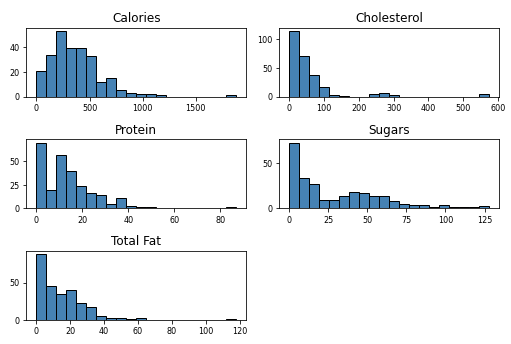
menu.hist(column=['Calories','Cholesterol','Sugars','Protein','Total Fat'],bins=20, color='steelblue', edgecolor='black', linewidth=1.0,
           xlabelsize=8, ylabelsize=8, grid=False) # historam for each attribute. adjust size and colors
plt.tight_layout(rect=(0, 0, 1.2, 1.2))
plt.ylabel("Counter") # naming the y-axis
plt.xlabel("Values") # naming the x-axis
Text(0.5, 0, 'Values')
So first we’ll import some libraries that will help us later to analyze.
sns.set(font_scale=1.4)
menu['Category'].value_counts().plot(kind='bar', figsize=(7, 6)) # makes plot bar for each category
plt.xlabel("Categories", labelpad=5) # title for the x label
plt.ylabel("Count of items", labelpad=5) # title for the y label
plt.title("Count of items by its category", y=1.02); # title for the plot
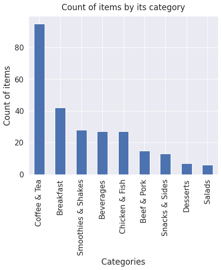
I see that the dishes are divided into categories. Here’s a look of the distribution along the categories. we can see that the biggest category is coffe & Tea, and the category with the lowest variety.
# Histogram
fig = plt.figure(figsize = (6,4)) # adjust plot for size
title = fig.suptitle("Calories of each item", fontsize=14) # title for plot
fig.subplots_adjust(top=0.85, wspace=0.3) # Tune the subplot layout. adjust the placing

ax = fig.add_subplot(1,1, 1) # adds subplot to the figure
ax.set_xlabel("Calories") # naming the x-axis
ax.set_ylabel("Frequency") # naming the y-axis
freq, bins, patches = ax.hist(menu['Calories'], color='steelblue', bins=30,
                                    edgecolor='black', linewidth=1) # histogram for each category of calories


# Density Plot
fig = plt.figure(figsize = (6, 4)) # adjust plot for size
title = fig.suptitle("Calories of each item", fontsize=14) # title for plot
fig.subplots_adjust(top=0.85, wspace=0.3) # Tune the subplot layout. adjust the placing

ax1 = fig.add_subplot(1,1, 1) # adds the 2nd subplot to the figure
ax1.set_xlabel("Calories") # naming the x-axis
ax1.set_ylabel("Frequency") # naming the y-axis
sns.kdeplot(menu['Calories'], ax=ax1, shade=True, color='steelblue')  # Fit and plot a univariate or bivariate kernel density estimate.
<matplotlib.axes._subplots.AxesSubplot at 0x7fe94fa778d0>
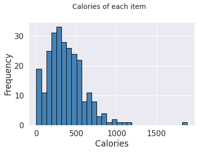
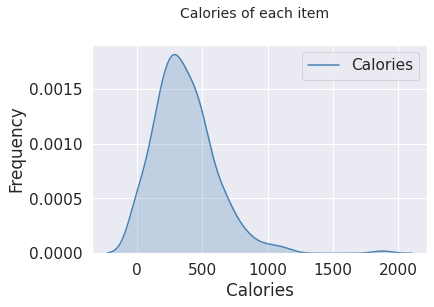
We can see that most of the items contain between 250-500 calories. There’s also one giant dish that is really exceptional. let’s check which one is it.
menu[menu['Calories']==menu['Calories'].max()]['Item'] # gets the highest-calorie dish
82    Chicken McNuggets (40 piece)
Name: Item, dtype: object
So we can see that the dish with the biggest calorie values is Chicken McNuggets (40 piece). keep away from it :)
sugars = menu['Sugars'] # sugars values column
calories = menu['Calories'] # calories values column
plt.scatter(calories, sugars) # scatter plot of calories vs sugars
plt.xlabel('calories') # naming the x-axis
plt.ylabel('sugars') naming the y-axis
plt.show()
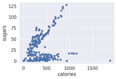
Here’s an interesting scatter plot, which is great to display correlation between two parameters. the x axis shows the calories and the y axis shows the sugars. we can see that there’s clear linear correlation between calories and sugars, as long as we have more calories in the dish, it contains more sugars, at most of the dishes. we can see some exceptionals at dishes between 0-750 calories that have maximum 25 grams of sugars.
menu.pivot_table('Trans Fat', 'Category').plot(kind='bar', stacked=True, color = 'c') # bar plot of each category and the mean of its Trans fat
<matplotlib.axes._subplots.AxesSubplot at 0x7fe94f781410>
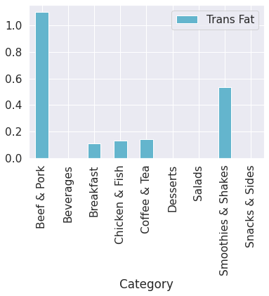
Well, the dishes with the most Trans Fat are Beef & Pork and Smoothies & Shakes.
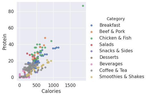
Protein = menu['Protein'] # protein column
Calories = menu['Calories'] # calories column
Category = menu['Category'] # category column

df = pd.DataFrame(dict(Calories=Calories, Protein=Protein, Category=Category)) # data frame of the 3 column
sns.lmplot('Calories', 'Protein', data=df, hue='Category', fit_reg=False) # Plot data of Calories vs Protein, based on categories by colors
plt.show()
cols = ['Calories','Cholesterol','Trans Fat','Sugars','Dietary Fiber']
cm = np.corrcoef(menu[cols].values.T) # Return Pearson product-moment correlation coefficients on all the columns
sns.set(font_scale = 1.5) # Set aesthetic parameters in one step.
hm = sns.heatmap(cm,cbar = True, annot = True,square = True, fmt = '.2f', annot_kws = {'size':15}, yticklabels = cols, xticklabels = cols) # correlation matrix between some main values
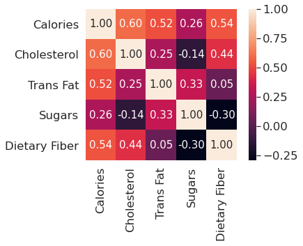
correlation matrix between some main values. Calories has positive correlation with Cholesterol and Trans Fat, and Sugars has negative correlation with Dietary Fiber.
def plot(grouped):
    item = grouped["Item"].sum() # group items by names
    item_list = item.sort_index() # sort the items by sugar values
    item_list = item_list[-20:] # keeps only the 20 first items
    plt.figure(figsize=(9,10))
    graph = sns.barplot(item_list.index,item_list.values) #x is the sugar values, y is the item name
    labels = [aj.get_text()[-40:] for aj in graph.get_yticklabels()] # crop text to make it look better
    graph.set_yticklabels(labels)
    sugar = menu.groupby(menu["Sugars"]) # group by sugars
    plot(sugar)
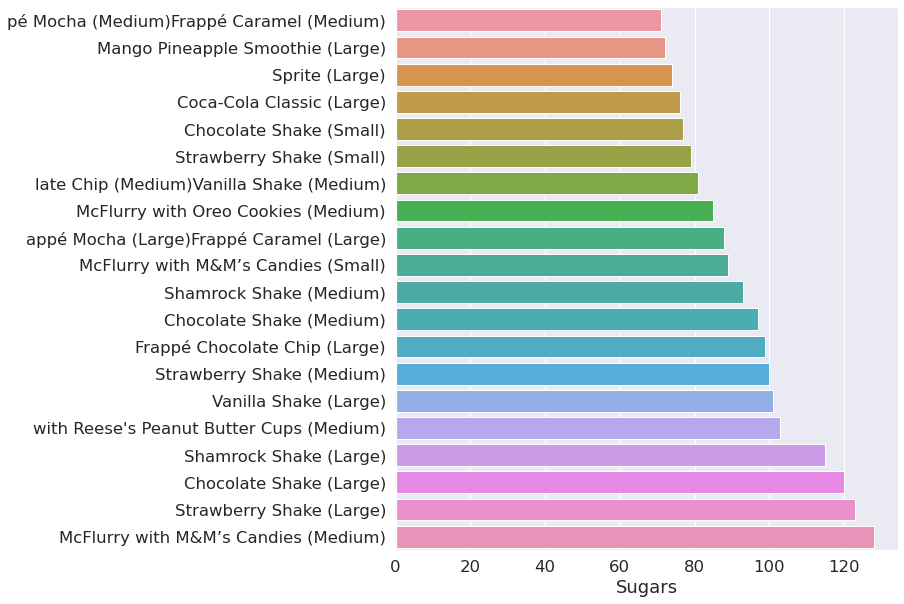
TOP 20 items by sugar.
protein = menu.groupby(menu["Protein"])
plot(protein)
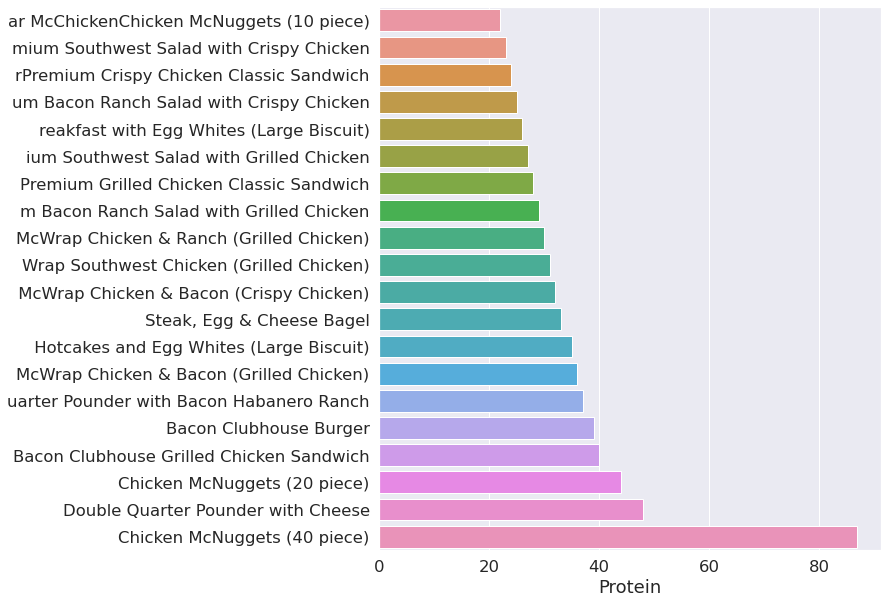
Top 20 items by Protein. so 40 Nuggets contains alot of Protein, but what with Cholsetrol and Fat? let’s see.
Cholesterol = menu.groupby(menu["Cholesterol"])
plot(Cholesterol)
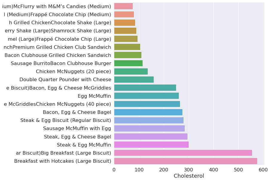
Top 20 items by cholesterol
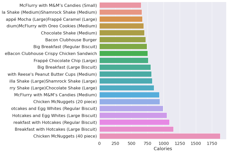
calories = menu.groupby(menu["Calories"])
plot(calories)
Saturated = menu.groupby(menu["Saturated Fat"])
plot(Saturated)
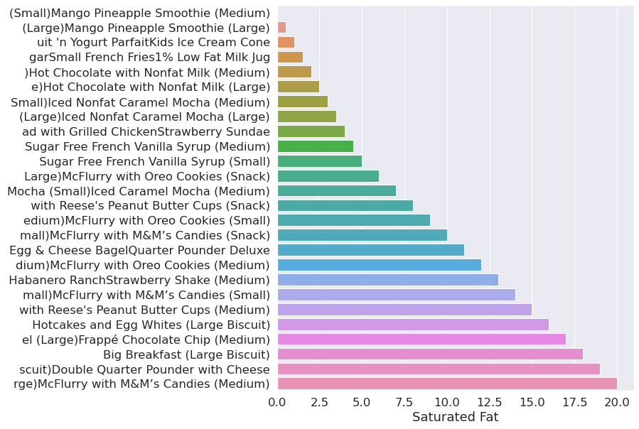
Top 20 items by calories.
menu.corr()['Calories'].sort_values()
Vitamin C (% Daily Value)       -0.068747
Vitamin A (% Daily Value)        0.108844
Sugars                           0.259598
Calcium (% Daily Value)          0.428426
Trans Fat                        0.522441
Dietary Fiber                    0.538894
Dietary Fiber (% Daily Value)    0.540014
Cholesterol (% Daily Value)      0.595208
Cholesterol                      0.596399
Iron (% Daily Value)             0.643552
Sodium                           0.712309
Sodium (% Daily Value)           0.713415
Carbohydrates (% Daily Value)    0.781242
Carbohydrates                    0.781539
Protein                          0.787847
Saturated Fat                    0.845564
Saturated Fat (% Daily Value)    0.847631
Total Fat (% Daily Value)        0.904123
Total Fat                        0.904409
Calories from Fat                0.904588
Calories                         1.000000
Name: Calories, dtype: float64
The method corr gives us correlation of specific column with all the other columns. in this example, we can see that calories has strong positive correlation with total fat, saturated fat, and carbohtydrates.
This Project was created as the Final Project in the Big Data Engineer course at Naya College By Nitay Yacobovitch, Shoham Gilady and Dor Izmaylov. We used M...
This post shows an analysis that I did of the solar system at my home - and its performaמce. It contains the total yield from the last 6 years - on top of t...
Recommendation on a great video, step by step instruction on creating interactive dashboard from scratch using the built in Excel tools.
This post shows an analysis that I’ve made of Mcdonalds Menu - The data i used holds information on all of the dishes from their menu, on top of that i made ...