Data Engineer Course Final Project - MBTA API
This Project was created as the Final Project in the Big Data Engineer course at Naya College By Nitay Yacobovitch, Shoham Gilady and Dor Izmaylov. We used M...

This post shows an analysis that I did of the solar system at my home - and its performaמce. It contains the total yield from the last 6 years - on top of that I made some data cleansing, showed few insights and provided graphs.
# This Python 3 environment comes with many helpful analytics libraries installed
# It is defined by the kaggle/python Docker image: https://github.com/kaggle/docker-python
# For example, here's several helpful packages to load

import numpy as np # linear algebra
import pandas as pd # data processing, CSV file I/O (e.g. pd.read_csv)
import seaborn as sns
import matplotlib.pyplot as plt

# Input data files are available in the read-only "../input/" directory
# For example, running this (by clicking run or pressing Shift+Enter) will list all files under the input directory

import os
for dirname, _, filenames in os.walk('/kaggle/input'):
    for filename in filenames:
        print(os.path.join(dirname, filename))

# You can write up to 5GB to the current directory (/kaggle/working/) that gets preserved as output when you create a version using "Save & Run All"
# You can also write temporary files to /kaggle/temp/, but they won't be saved outside of the current session
/kaggle/input/annualcomparisonsolarsystem/Annual_Comparison_2020_07_04.csv
solar = pd.read_csv("/kaggle/input/annualcomparisonsolarsystem/Annual_Comparison_2020_07_04.csv") # the solar dataset is now a Pandas
solar.head()
solar = solar.dropna(subset=['Total yield [kWh]'])
print(solar.to_string())
   Total yield [kWh]  January  February    March    April      May     June     July   August  September  October  November  December     Total
0             2014.0      NaN       NaN      NaN      NaN   780.67  2967.07  3050.46  2817.26    2329.23  1858.61   1537.28   1542.12  16882.69
1             2015.0  1427.24   1580.28  2350.50  2495.05  2880.93  2790.83  3017.52  2742.42    2235.77  1824.12   1479.86   1541.99  26366.50
2             2016.0  1312.06       NaN      NaN      NaN      NaN      NaN   922.20  2553.03    2339.24  2014.08   1571.30   1337.75  12049.67
3             2017.0  1484.67   1679.77  2016.53  2469.81  2707.03  2562.49  2514.67  2719.89    2340.79  1921.68   1437.16   1183.86  25038.34
4             2018.0  1227.53   1537.83  2304.27  2434.25  2264.23  2450.22  1781.75  2051.28    1888.90  1470.56       NaN       NaN  19410.81
5             2019.0  1383.32   1499.07  1894.44  2311.29  2593.29  2460.69  2532.43  2505.71    1353.53  1193.87   1224.51   1017.01  21969.15
6             2020.0   921.59   1043.50  1445.02  1730.01  2118.69  2121.16   215.72      NaN        NaN      NaN       NaN       NaN   9595.68
cols = ['January','February','March', 'April', 'May', 'June','July', 'August', 'September', 'October', 'November', 'December' ]
solar[cols] = solar[cols].fillna(solar[cols].mean()) #Calculates nan values for the mean of the same column (the same month allover the years)
df = solar.melt(id_vars=["Total yield [kWh]"],
        var_name="Month",
        value_name="Value")
df = df.rename(columns={'Total yield [kWh]': 'Year', 'Value': 'Value'})
df = df.dropna(subset=['Year'])


print(df.to_string())
      Year      Month         Value
0   2014.0    January   1292.735000
1   2015.0    January   1427.240000
2   2016.0    January   1312.060000
3   2017.0    January   1484.670000
4   2018.0    January   1227.530000
5   2019.0    January   1383.320000
6   2020.0    January    921.590000
7   2014.0   February   1468.090000
8   2015.0   February   1580.280000
9   2016.0   February   1468.090000
10  2017.0   February   1679.770000
11  2018.0   February   1537.830000
12  2019.0   February   1499.070000
13  2020.0   February   1043.500000
14  2014.0      March   2002.152000
15  2015.0      March   2350.500000
16  2016.0      March   2002.152000
17  2017.0      March   2016.530000
18  2018.0      March   2304.270000
19  2019.0      March   1894.440000
20  2020.0      March   1445.020000
21  2014.0      April   2288.082000
22  2015.0      April   2495.050000
23  2016.0      April   2288.082000
24  2017.0      April   2469.810000
25  2018.0      April   2434.250000
26  2019.0      April   2311.290000
27  2020.0      April   1730.010000
28  2014.0        May    780.670000
29  2015.0        May   2880.930000
30  2016.0        May   2224.140000
31  2017.0        May   2707.030000
32  2018.0        May   2264.230000
33  2019.0        May   2593.290000
34  2020.0        May   2118.690000
35  2014.0       June   2967.070000
36  2015.0       June   2790.830000
37  2016.0       June   2558.743333
38  2017.0       June   2562.490000
39  2018.0       June   2450.220000
40  2019.0       June   2460.690000
41  2020.0       June   2121.160000
42  2014.0       July   3050.460000
43  2015.0       July   3017.520000
44  2016.0       July    922.200000
45  2017.0       July   2514.670000
46  2018.0       July   1781.750000
47  2019.0       July   2532.430000
48  2020.0       July    215.720000
49  2014.0     August   2817.260000
50  2015.0     August   2742.420000
51  2016.0     August   2553.030000
52  2017.0     August   2719.890000
53  2018.0     August   2051.280000
54  2019.0     August   2505.710000
55  2020.0     August   2564.931667
56  2014.0  September   2329.230000
57  2015.0  September   2235.770000
58  2016.0  September   2339.240000
59  2017.0  September   2340.790000
60  2018.0  September   1888.900000
61  2019.0  September   1353.530000
62  2020.0  September   2081.243333
63  2014.0    October   1858.610000
64  2015.0    October   1824.120000
65  2016.0    October   2014.080000
66  2017.0    October   1921.680000
67  2018.0    October   1470.560000
68  2019.0    October   1193.870000
69  2020.0    October   1713.820000
70  2014.0   November   1537.280000
71  2015.0   November   1479.860000
72  2016.0   November   1571.300000
73  2017.0   November   1437.160000
74  2018.0   November   1450.022000
75  2019.0   November   1224.510000
76  2020.0   November   1450.022000
77  2014.0   December   1542.120000
78  2015.0   December   1541.990000
79  2016.0   December   1337.750000
80  2017.0   December   1183.860000
81  2018.0   December   1324.546000
82  2019.0   December   1017.010000
83  2020.0   December   1324.546000
84  2014.0      Total  16882.690000
85  2015.0      Total  26366.500000
86  2016.0      Total  12049.670000
87  2017.0      Total  25038.340000
88  2018.0      Total  19410.810000
89  2019.0      Total  21969.150000
90  2020.0      Total   9595.680000
boxplot = df.boxplot(by='Year',figsize=(12,12),showfliers=False)
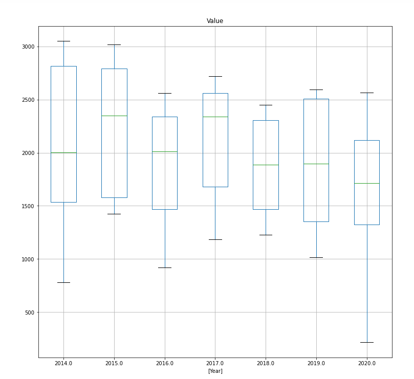
print(df.groupby(['Year']).mean())
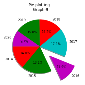
cols = ['r','g','m','c']
slices =[3,5,7,5]
activities=["2014","2015","2016","2017","2018","2019","2020"]
# explode()- Helps to extract the particular piece out.
# autopct='%1.1f%%' helps to add a percentage to the pie chart
plt.pie(df.groupby(['Year']).mean(), labels=activities, colors = cols,shadow =True,
startangle =180,explode =(0,0,0.5,0,0,0,0),autopct='%1.1f%%')
plt.title('Pie plotting \n Graph-9')
plt.show()
              Value
Year
2014.0  3139.726846
2015.0  4056.385385
2016.0  2664.656718
2017.0  3852.053077
2018.0  3199.707538
2019.0  3379.870000
2020.0  2178.917923


/opt/conda/lib/python3.7/site-packages/ipykernel_launcher.py:9: MatplotlibDeprecationWarning: Non-1D inputs to pie() are currently squeeze()d, but this behavior is deprecated since 3.1 and will be removed in 3.3; pass a 1D array instead.
  if __name__ == '__main__':
This Project was created as the Final Project in the Big Data Engineer course at Naya College By Nitay Yacobovitch, Shoham Gilady and Dor Izmaylov. We used M...
This post shows an analysis that I did of the solar system at my home - and its performaמce. It contains the total yield from the last 6 years - on top of t...
Recommendation on a great video, step by step instruction on creating interactive dashboard from scratch using the built in Excel tools.
This post shows an analysis that I’ve made of Mcdonalds Menu - The data i used holds information on all of the dishes from their menu, on top of that i made ...